Predictive maintenance IoT: calculating real ROI before you invest

Predictive Maintenance (PdM) for the Internet of Things (IoT) instruments a critical machine with vibration, temperature and current sensors to anticipate failure several weeks ahead and produce a measurable Return on Investment (RoI). At AESTECHNO, an electronic design house based in Montpellier, we design sensors compliant with ISO 10816, with a 6-step framework to validate profitability before committing to 3 to 5 years of deployment.

Contents

• Predictive vs reactive vs preventive maintenance: financial impact
• ROI calculation framework: 6 steps to avoid mistakes
• The false-positive trap: alert fatigue
• POC strategy to minimise risk
• Lab cases we have seen
• Vibration standards and validation tools
• Which radio network for predictive maintenance?
• Data quality: the forgotten prerequisite
• In short

Predictive vs reactive vs preventive maintenance: financial impact

Predictive maintenance is a condition-based strategy that fires an intervention only when measured sensor data crosses a validated threshold, whereas preventive maintenance is a calendar-based strategy and reactive maintenance is a post-failure strategy. Predictive maintenance triggers an intervention based on a measured vibration or thermal signature, unlike preventive maintenance which follows a fixed calendar (2000 h) and reactive maintenance which waits for failure. These three strategies are judged on three standard KPIs: MTBF (Mean Time Between Failures), MTTR (Mean Time To Repair) and OEE (Overall Equipment Effectiveness, reference target ≥ 85%).

1. Reactive (or corrective) maintenance

Principle: repair when it breaks, with no prior monitoring of machine state.

Typical costs for a critical machine:

• Emergency parts: +30 to 50 % vs. normal price (express freight, supplier surcharge)
• Technician intervention: 2 to 5× more expensive (overtime, immediate dispatch)
• Production downtime: 8 to 72 hours (waiting for parts, diagnosis, repair)
• Collateral damage: a broken bearing can destroy the motor shaft (cascading failures)

MTTR impact: typically 4 to 8× the MTTR of a planned preventive intervention, with a direct effect on OEE.

2. Preventive maintenance (fixed planning)

Principle: change parts on a calendar (for example every 2000 h).

Typical costs:

• New parts: premature replacement (the part still has 60 % life left)
• Planned downtime: 4 to 8 h of lost production per intervention
• Labour: normal cost (planned intervention)
• Waste: 30 to 40 % of parts replaced prematurely

Advantage: no surprise failures, but a high cost in parts and planned downtime.

3. Predictive maintenance (based on actual condition)

Principle: intervene when sensors detect degradation, typically a vibration RMS above the ISO 10816-3 threshold (for example 4.5 mm/s for a Class II machine or 7.1 mm/s for Class III), or a thermal drift greater than 10 °C from the nominal hotspot, measured with typical accuracy of ±1 °C. These severity classes, according to Siemens industrial reliability guidance, align with the shaft height and mounting type as codified in IEC 60034-14 by the IEC, which is why a serious programme never uses a single threshold for the whole fleet.

Typical promises (according to McKinsey in its 2025 operations survey):

• Downtime reduction: -40 to 50 % (McKinsey, 2025)
• Maintenance cost reduction: -25 to 30 %
• Equipment lifetime increase: +20 to 25 %
• Spare parts stock optimisation: -15 to 20 % (anticipated needs)

But beware: these numbers are optimistic averages. Reality depends on your context (machine types, data quality, organisational maturity).

ROI calculation framework: 6 steps to avoid mistakes

A Return on Investment (RoI) framework is a sequenced calculation that ties each technical choice to a monetary baseline, so a predictive-maintenance project is evaluated against real downtime cost rather than vendor marketing.

Step 1: Calculate the real cost of your current failures

Don’t trust your intuition. Analyse your last 12-24 months with this formula:

Annual failure cost = (Number of failures × Average downtime × Hourly production cost) + Emergency repair costs

Example: 50-machine workshop:

• Failures/year: 18 critical failures
• Average downtime: 16 hours
• Hourly cost of lost production: 4,500 €/h (hourly revenue minus variable costs)
• Emergency repair costs: 280,000 €/year

Total = (18 × 16 × 4,500) + 280,000 = 1,296,000 + 280,000 = 1,576,000 €/year

Common mistake: forgetting indirect costs (customer delays, contractual penalties, brand damage).

Step 2: Identify critical machines (Pareto principle)

In 80 % of cases, 20 % of your machines cause 80 % of the downtime. Focus on them first.

Criticality criteria:

1. Bottleneck: if this machine stops, the whole line stops
2. Repair time: >8h (rare parts, specialised skills)
3. Failure history: >3 failures/year costing >20k€ each
4. Equipment age: >10 years (accelerated degradation)

Result: on 50 machines, you identify 8-12 critical machines to instrument first.

Step 3: Size the sensors (avoid over-instrumentation)

Not every sensor is needed on every machine. Here is the minimum viable set:

Machine type	Essential sensors	Unit cost
Rotating motors	Vibration (3-axis) + temperature	800-1,200 €
Pumps	Vibration + pressure + flow	1,200-1,800 €
Compressors	Vibration + temperature + motor current	1,500-2,200 €
Conveyors	Vibration (single-axis) + temperature	600-900 €
Transformers	Temperature (multi-point) + dissolved gas	2,000-3,500 €

For 10 critical machines (typical mix): sensor budget = 12,000 – 18,000 €

In sectors exposed to physical risks (steel, chemicals, construction), predictive maintenance also extends to operator monitoring: wearable devices integrating biometric sensors (heart rate, body temperature, fall-detection accelerometer) help prevent accidents linked to fatigue or thermal stress, complementing machine monitoring.

Step 4: Calculate full costs (infrastructure + platform + integration)

Initial costs (CAPEX):

• Sensors: 12,000 – 18,000 € (10 machines)
• IoT gateways: 3,000 – 6,000 € (2-4 gateways depending on surface area)
• Analytics platform: 15,000 – 50,000 € (licence + configuration)
• Installation + cabling: 8,000 – 15,000 €
• Team training: 5,000 – 10,000 €
• CMMS integration: 10,000 – 25,000 € (if connecting ERP/CMMS)

Total CAPEX: 53,000 – 124,000 € for 10 machines

Recurring costs (annual OPEX):

• Cloud platform subscription: 8,000 – 20,000 €/year
• Connectivity: 1,200 – 3,000 €/year (cellular or private LoRaWAN)
• Technical support: 5,000 – 12,000 €/year
• Sensor maintenance: 2,000 – 4,000 €/year (recalibration, replacement)

Total OPEX: 16,200 – 39,000 €/year

For systems deployed in areas without cellular coverage or that need maximum autonomy, the radio protocol choice directly impacts OPEX. Our article on NB-IoT, LTE-M and satellite connectivity details the options for keeping data flowing in isolated environments, including satellite solutions for remote industrial sites.

Step 5: Estimate realistic gains (not marketing promises)

Conservative scenario (prudent for ROI validation):

• Downtime reduction: -25% (not -50%) → 324,000 €/year savings
• Emergency repairs reduction: -20% → 56,000 €/year savings
• Spare parts stock optimisation: -10% → 15,000 €/year savings

Total conservative annual gains: 395,000 €/year

Note: in year one, count only 60-70 % of these gains (algorithm learning time, threshold adjustments).

Step 6: Calculate ROI and payback period

Year 1:

• Initial investment: -90,000 € (average CAPEX)
• OPEX: -25,000 €
• Gains (70% of potential): +276,500 €
• Net result: +161,500 €

Year 1 ROI = (161,500 / 90,000) × 100 = 179%

Payback period = 90,000 / 276,500 ≈ 4 months

Years 2-5:

• Annual OPEX: -25,000 €
• Gains (100% of potential): +395,000 €
• Net benefit/year: +370,000 €

Cumulative 5-year ROI = (161,500 + 4×370,000 – 90,000) / 90,000 = 1,750%

The false-positive trap: the hidden cost of alert fatigue

Alert fatigue is the operational state in which a monitoring system produces so many false positives that technicians ignore real warnings, and it is the single most under-estimated cost of predictive-maintenance deployments. A major issue rarely mentioned: false alerts.

Real scenario: your system generates 150 alerts/month. After investigation:

• 15 valid alerts (10 %): justified intervention
• 135 false-positive alerts (90 %): wasted technician time

Cost of false positives:

• Investigation time: 135 × 1 h = 135 h/month
• Technician hourly cost: 45 €/h
• Monthly loss: 6,075 € = 72,900 €/year

This cost cancels 18 % of your gains if not controlled.

Solutions:

1. Learning phase: 3-6 months to refine alert thresholds
2. Adaptive Machine Learning: algorithms that learn each machine’s normal behaviour
3. Alert prioritisation: low/medium/high criticality (don’t disturb for everything)
4. Visual dashboards: technicians see the trend before the alert fires

POC (Proof of Concept) strategy: minimise risk

A Proof of Concept (POC) is a bounded pilot deployment on one or two machines that validates the full sensor-to-dashboard chain before any fleet-wide rollout. Never deploy on 50 machines at once. Use a progressive approach:

Phase 1: POC on 1 machine (2-3 months) – Budget 8,000-15,000 €

• Pick THE most problematic machine (with documented failure history)
• Install vibration + temperature sensors as a minimum
• Test the platform with one user (maintenance manager)
• Goal: validate that the system detects real anomalies

Success criterion: at least 1 failure avoided with 3 months of savings > POC cost.

Phase 2: deploy on 10 critical machines (6 months) – Budget 50-80k€

• Instrument the 10 machines identified in Step 2
• CMMS/ERP integration
• Wider maintenance team training
• Goal: positive ROI from 8-12 months

Phase 3: scale to 50+ machines (12-18 months) – Budget 150-300k€

• Extension to the rest of the fleet if Phase 2 succeeded
• Continuous algorithm optimisation
• Goal: cumulative gains >1M€ over 3 years

Our sensor and connectivity expertise for predictive maintenance

High-frequency, low-power vibration sensor: on a recent project, we deployed the STMicroelectronics IIS3DWB, a 3-axis accelerometer combining wide bandwidth (flat response up to 6 kHz) and very low operating current. The part, per STMicroelectronics datasheet DS12517 (ST product page), holds a 0.026 mg/sqrt(Hz) noise density, which is what lets it surface Ball Pass Frequency Inner-race harmonics that cheaper MEMS parts flatten. This “high-frequency + low-power” combination is decisive in vibration monitoring: it lets us extract usable signatures from bearings and gears while keeping multi-year battery life. Wide-band acceleration beyond 5 kHz, according to Bosch Rexroth field guidance, is where incipient bearing defects surface weeks before audible symptoms.

Battery and BMS, autonomy of remote sensors: a sensor installed on a distant motor only has value if it transmits for the full duration of a maintenance contract. At AESTECHNO we have shipped a broad portfolio of products integrating batteries and BMS (Battery Management System): protection, cell balancing, fuel gauge, RF current-peak management. This expertise determines whether real-world autonomy holds up over 5 to 10 years.

Full wireless portfolio: our portfolio covers every wireless technology deployed in customer projects. We ship Bluetooth (Classic, BLE, 5.4 PAwR), Wi-Fi, LoRa/LoRaWAN, RFID, 5G and LTE-M. Site architecture drives the choice. Dense indoor favours Bluetooth or Wi-Fi. Kilometre-scale outdoor favours LoRaWAN or cellular. Mobility favours LTE-M. We design dual-mode sensors when a single radio cannot cover the use case.

Data layer, top-tier HA cluster: we have designed and deployed a top-tier HA database cluster dedicated to massive IoT ingestion. A data gap equals an ML model blind exactly when a failure signature emerges. In our practice, what kills a project is not write latency. It is what happens when a node falls over at 3 a.m. with 50,000 sensors emitting. Multi-node replication, automatic failover and retention guarantee the continuity of the analytical flow.

Firmware CI/CD for deployed fleets: on several customer projects, we have built auto-deployment pipelines gated by tests to continuously push firmware updates to sensors in production. Principle: the pipeline is the only path to production. Each OTA binary pushed to field devices is signed, versioned and traceable to an auditable commit, essential when the fleet grows and algorithmic fixes must reach the field without regressions.

End-to-end IoT, rare on the market: end-to-end coverage under a single team is uncommon. The chain includes sensor hardware, firmware, connectivity, CI/CD and HA database. Reliable predictive maintenance requires every link to hold. An accurate sensor. A stable radio link. A data point that arrives. A data point that stays. A model that can be updated.

Lab cases we have seen

The following cases are concrete observations from recent client project work, where each situation illustrates a specific lever that separates a textbook architecture from one that actually performs in the field. Three situations from real projects illustrate where a predictive-maintenance architecture really creates value:

• Case 1: early bearing signature with the IIS3DWB. On a motor-characterisation bench, the STMicroelectronics IIS3DWB vibration sensor, sampled in wide band, identified a Ball Pass Frequency Inner-race (BPFI) harmonic component several weeks before the failure became perceptible to human maintenance. Against the intuition that pushes teams toward cheap narrowband sensors, we systematically recommend wide bandwidth on critical machines, the useful signal is often beyond the first harmonics.
• Case 2: fleet synchronisation in Bluetooth 5.4 PAwR. On a wireless-sensor deployment in an industrial environment, we characterised Periodic Advertising with Responses (PAwR) on Bluetooth Low Energy (BLE) 5.4, about a hundred devices synchronised with sub-5 µs sync, no collisions, and no Wi-Fi infrastructure. The reference stack, according to Nordic Semiconductor (nRF54L15 product brief), schedules PAwR response slots with deterministic jitter under 10 µs, which is exactly what synchronous vibration capture across a large fleet needs. Unlike LoRaWAN or cellular, PAwR delivers a controlled topology with bounded latency.
• Case 3: data flow holding up at 3 a.m. We deployed a top-tier HA database cluster for continuous sensor ingestion. Unlike marketing demos that highlight write latency, the real test is what happens when a node falls over at 3 a.m. with 50,000 sensors emitting. Multi-node replication, automatic failover and long retention guarantee that no failure signature is lost when it counts.

Which radio network for predictive maintenance?

The radio network is the wireless link that carries sensor data from the machine to the analytics platform. Its choice directly drives sensor autonomy and project Operational Expenditure (OPEX). The field data, according to Ericsson Mobility Report figures on Low Power Wide Area Network (LPWAN) deployments, shows no single radio wins on all three axes of range, throughput and power; the IEEE Communications Magazine surveys reach the same conclusion, which is why we arbitrate systematically between three families based on site density, gateway distance, and useful throughput:

• LoRaWAN: 2 to 5 km urban range, 10 to 15 km rural, 0.3 to 50 kbps throughput, typical sensor autonomy 3 to 5 years at one measurement/min on an AA cell. Ideal for slow readings (temperature, counting, aggregated vibration RMS) and large sites without cellular coverage. Details in our article LoRaWAN vs NB-IoT vs Sigfox.
• NB-IoT / LTE-M: cellular-operator coverage, 1.6 to 10 s latency, 20 to 250 kbps throughput, shorter autonomy than LoRaWAN but zero infrastructure to deploy. Application-layer protocols on top are typically MQTT or CoAP, both standardised and broker-friendly. Preferred when no gateway can be installed.
• Wi-Fi 6 / Bluetooth 5.4 PAwR: ≥ 1 Mbps throughput, < 10 ms latency, higher consumption so wired power or generous battery is required. We use it when monitoring requires uncompressed wide-band vibration signature capture (≥ 6 kHz).

MEMS vs piezoelectric comparison for the vibration chain: a modern MEMS accelerometer (such as the ST IIS3DWB) offers up to 6 kHz of flat band, sub-mA consumption, and a much lower cost; industrial piezoelectric sensors reach beyond 20 kHz and tolerate temperatures up to 150 °C, but require an IEPE conditioner and wired power. For 80 % of industrial rotating machines in Class II or III ISO 10816, wide-band MEMS is sufficient and radically simplifies wireless integration.

Vibration standards and validation tools

Vibration standards are the public reference grids that define when a rotating machine is “good”, “acceptable” or “unacceptable” based on measured RMS velocity. Published by the International Organization for Standardization (ISO), these documents turn a raw sensor reading into an actionable maintenance decision. A serious industrial predictive-maintenance project relies on this recognised framework, not on improvised thresholds:

• ISO 10816 (mechanical vibration, evaluation by measurement on non-rotating parts): defines vibration severity classes by machine power and type
• ISO 13374 (condition monitoring and diagnostics): functional architecture of condition monitoring systems
• ISO 17359: general guidelines for setting up a monitoring programme
• ISO 13379: data interpretation and diagnosis

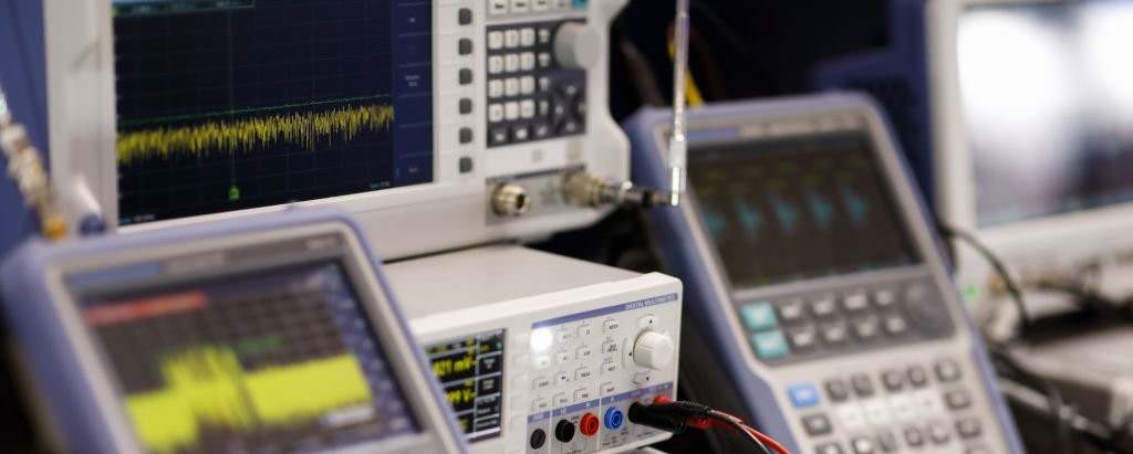
For tooling, we use the Nordic PPK2 and the Keithley DMM7510 in our lab to finely characterise wireless sensor consumption. In our lab we measured a 7 µA parasitic on an early IIS3DWB breakout. The fix was a single firmware pull-up reconfigured at boot. A predictive-maintenance RoI collapses if sensors must be replaced more often than the bearings they monitor. Nanopower regulators such as the TPS62840, according to Texas Instruments application note SLVA908 (TI TPS62840 resources), hold quiescent current below 60 nA, which is what keeps the sensor budget honest at the microamp level.

Unlike marketing RoI claims showing returns in 6 months, the real predictive-maintenance RoI rarely emerges before 18 to 24 months. ML models need time to accumulate history. False positives take 3 to 6 months to calibrate. Field teams need weeks to fold alerts into their rounds. In our practice, the curve really inverts in years 2 and 3, not in the first twelve months.

Data quality: the often-forgotten prerequisite

Data quality is the precondition on which every Machine Learning (ML) model is built, and a predictive-maintenance algorithm is only as trustworthy as the historical dataset that trains it. ML algorithms need clean historical data:

Minimum required data:

• 6-12 months of failure history: dates, causes, parts changed, downtime
• Up-to-date maintenance log: preventive interventions performed
• Machine parameters: rotation speed, load, normal temperature

If your data is missing or incomplete:

• Add 3 to 6 months of data collection before AI is effective
• Plan budget to digitise and structure existing data
• Start with simple rules (fixed thresholds) before advanced ML

In short: what separates a profitable project from a failed one

A profitable predictive-maintenance project is one where sensor choice, radio sizing and data continuity all hold at once. An IoT predictive maintenance project becomes profitable when three disciplines hold simultaneously: a fit-for-purpose sensor (wide-band MEMS for ≥ 80 % of Class II ISO 10816 rotating machines, IEPE piezo above), a properly sized radio (LoRaWAN for 2 to 15 km with 3 to 5 years autonomy; NB-IoT/LTE-M cellular without a gateway; Bluetooth 5.4 PAwR for wide-band signatures), and a continuous data layer (HA cluster, replication, backfill). Unlike marketing ROI claims of 6 months, our field experience frames the real curve over 18 to 24 months, with the first year at 60-70 % of potential while ML models learn and false positives are calibrated.

At AESTECHNO, an electronic design house based in Montpellier, we design the full chain: ISO 10816-compliant MEMS/piezo sensor, low-power RTOS firmware, BMS for multi-year autonomy, HA backend so no failure signature is lost. This full-stack coverage under a single engineering team is rare on the market, and it is precisely what avoids the three classic failures: a poorly placed sensor, a saturated radio link, a data point lost just as a failure signature emerges.

FAQ: predictive maintenance IoT and ROI

What is the difference between predictive maintenance and condition monitoring?
Condition monitoring is one component of this approach. It collects sensor data continuously (vibration, temperature), while the predictive layer adds intelligence (AI, ML) to predict when a failure will happen (in 2 weeks, 1 month). AESTECHNO integrates both: real-time monitoring + algorithms tuned to your machines.

How long does it take for AI algorithms to become reliable?
Count 3-6 months minimum of data collection so Machine Learning learns each machine’s normal patterns. For complex equipment (turbines, high-pressure compressors), allow 12 months. During that period, use fixed thresholds validated by your maintenance experts. Our electronic design house in Montpellier combines domain expertise and AI to accelerate the ramp-up.

Can predictive maintenance work without cloud (edge computing only)?
Yes, with an edge computing architecture where processing happens locally on industrial gateways. Pros: no internet dependency, ultra-low latency (<100 ms), guaranteed data confidentiality. Cons: +20-30 % initial cost (more powerful edge hardware), less flexibility to adjust models. We recommend an edge + cloud mix: real-time processing local, long-term storage and AI re-training in the cloud.

What are the main organisational obstacles to deployment?
From our field experience: (1) resistance from senior technicians who fear being replaced by AI → solution: position them as experts who validate alerts; (2) lack of data skills → internal training or external partner; (3) silos between IT and maintenance → create a cross-functional project team from day one. Success depends on people as much as technology.

Does this approach work for every industry?
Particularly profitable for: petrochemicals (downtime = millions €/day), food processing (contamination on failure), automotive (just-in-time), energy (critical availability). Less relevant for: small batches, simple low-cost machines, artisanal environments. Rule of thumb: if one hour of downtime costs >2,000€, the investment is probably justified. AESTECHNO runs a free feasibility audit to validate your use case.

Related

The articles below are companion references that complete the predictive-maintenance stack, from radio layer choice to IoT cybersecurity and robust sensor design. To complete your IoT predictive maintenance strategy:

• LoRaWAN, NB-IoT, Sigfox: which network for your sensors? – Pick the right connectivity for your plant (range, cost, autonomy)
• Which IoT database for your sensors? – Store and exploit machine time-series (InfluxDB, TimescaleDB)
• Industrial IoT cybersecurity: threats and solutions – Protect your sensors and production data against attacks
• Electronic board design: method & industrialisation – How we design certified, robust industrial sensors